Predicting Stock Prices using Machine Learning

10 min readMar 14, 2021

Time Series Forecasting

Problem

Investment firms, hedge funds and even individuals have been using financial models to better understand market behavior and make profitable investments and trades. A wealth of information is available in the form of historical stock prices and company performance data, suitable for machine learning algorithms to process.

In this article, we will use a machine learning driven approach to build a stock price predictor that takes daily trading data over a certain date range as input, and outputs projected estimates for different time ranges in the future. Note that the inputs will contain multiple metrics, such as opening price (Open), highest price the stock traded at (High), how many stocks were traded (Volume) and closing price adjusted for stock splits and dividends (Adjusted Close). Our model only needs to predict the Adjusted Close price.

Since the stock market data is a time series, we will explore regression and neural networks models to try to accurately predict the future value of the stock. We will evaluate our predictions on test data looking at both mean absolute error and root mean squared (RMS) error.

Analysis

Historical Stock Data

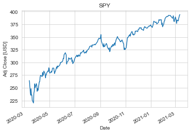
We will use the S&P 500 ETF (listed as ‘SPY’ on the stock market) historical data for analysis. The S&P 500 serves as a good benchmark as most stock prices tend to follow the momentum of the market. We obtain the historical data we need from Yahoo using the pandas-datareader:

stock = 'SPY'df = web.DataReader(stock, data_source='yahoo', start=start_date, end=end_date)

Taking a look at the data, we can see that we only have information for the days when the stock market was open. This excludes weekends and holidays.

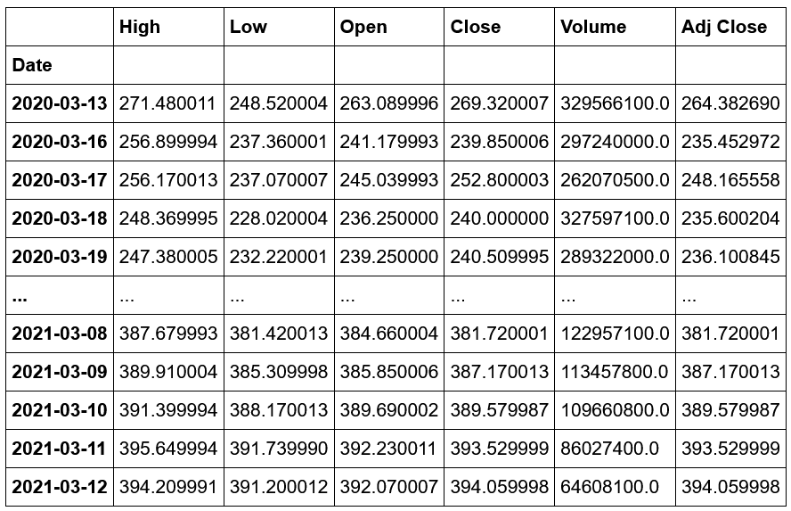
However, it’s always a good idea to do a sanity check for null values. I didn’t find any null values in the data I pulled. In case you do, a quick fix would be to do a forward fill followed by a backward fill.

df.isnull().sum()  # check for null values

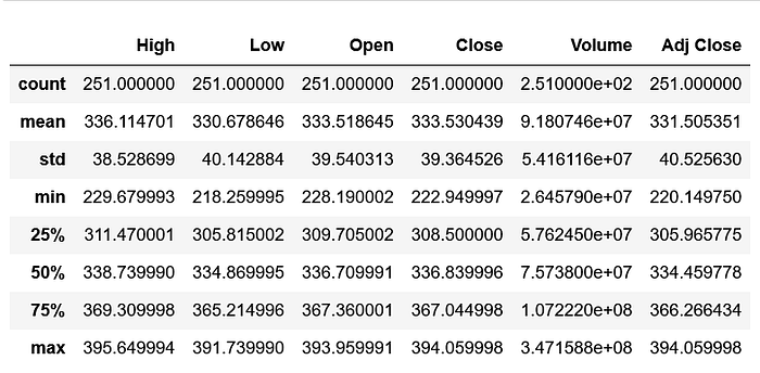
We have 6 columns in our data: highest price the stock traded at (High), lowest price the stock traded at (Low), opening price (Open), closing price (Close), how many stocks were traded (Volume) and closing price adjusted for stock splits and dividends (Adjusted Close). It’s always a good practice to look at the summary of the data. This will give you a sense of the different ranges for each of the columns. We have 251 days of ‘SPY’ stock data for the last year.

Our goal is to predict a future Adjusted Close value for each trading day. This could be 1 day in the future, 14 days or as many days as you’d like. We create a new column called Future, which holds the Adjusted Close value n days into the future.

df['Future'] = df['Adj Close'].shift(-n)

Here’s the updated table with Future value added. In this table, we have chosen n to be 28 days.

Features and Labels

For our model, we use all columns except the Future value as our features, and the Future value becomes the label we will train our model to predict.

X = df.drop('Future', axis=1).iloc[:-n]  # featuresy = df['Future'].iloc[:-n]  # label

Algorithms

We will take a look at 2 main approaches to predict the SPY future price:

Regression
Long Short-Term Memory network (LSTM)

Train Test Split

Since we are working with time series data here, the data is split into training and test sets sequentially. In other words, we train using data upto a particular date and then predict on data past that date.

X_train = X.iloc[:split_index]y_train = y.iloc[:split_index]X_test = X.iloc[split_index:]y_test = y.iloc[split_index:]

Implementation

Regression

We look at 2 regression models by trying to predict adjusted close values 28 days into the future:

Decision Tree Regressor: We use scikit learn’s decision tree regressor.

model = DecisionTreeRegressor()model.fit(X_train, y_train)  # train modely_pred = model.predict(X_test)  # make predictions on test dataset

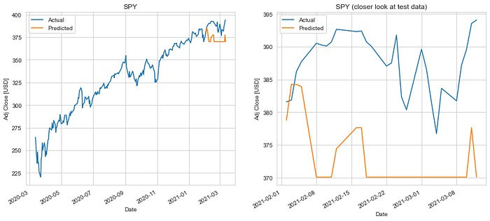
The decision tree regression model did not do a good job in predicting future stock price value on the test set. We ended up with a mean absolute error of $14.81 and a RMS error of $16.08.

Decision trees do not have the natural ability to deal with time series data. This is mainly because it cannot do extrapolation being a classifier. Hence, we will focus our efforts on Linear Regression and LSTM neural network.

Linear Regression: We use scikit learn’s linear regression.

model = LinearRegression()model.fit(X_train, y_train)  # train modely_pred = model.predict(X_test)  # make predictions on test dataset

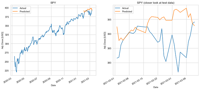
The linear regression model performed much better, giving us a mean absolute error of $6.70 and a RMS error of $9.00.

Long Short-Term Memory network (LSTM)

In this section, we will focus on building a LSTM neural network to predict a 28 days future price. The LSTM model will learn a function that maps a sequence of past observations as input to an output observation, which is predicted adjusted close value in our case.

Data Preprocessing

Let’s start by preparing the data. Since we are using a neural network model, it is good practice to scale the data. We use sklearn’s MinMaxScaler to scale each feature to range (0,1).

cols = list(df.columns)scaler = MinMaxScaler()df_scaled = scaler.fit_transform(df[cols])

Features and Label

Our features here are a series of features chosen earlier and our label is still the future value we will train our model to predict. In simple words, we need past m days feature data to predict adjusted close value n days into the future.

X = []  # featuresy = []  # labelfor i in range(m, len(df_scaled) - n + 1):X.append(df_scaled[i - m:i, :-1])y.append(df_scaled[i - 1, -1])

The shape of X would be: Number of rows x m x 6 (The 6 here is from 6 columns in the data frame excluding Future column.)

The shape of y would be: Number of rows x 1

After we have X and y arrays, we can slice the data to split it into train and test sets. Additionally, we reshape the array to have their shape properly defined to pass through the neural network.

Build the Model

We then go ahead and build the LSTM neural network model. Firstly, we add in 2 LSTM layers, the first with 64 neurons and the second with 32 neurons. Secondly, we add a dropout layer to prevent overfitting. Finally, we have 2 dense layers of which the last one will output the scaled stock price prediction.

model = Sequential()model.add(LSTM(64, input_shape=(X_train.shape[1], X_train.shape[2]), return_sequences=True))model.add(LSTM(32, return_sequences=False))model.add(Dropout(0.2))model.add(Dense(16))model.add(Dense(y_train.shape[1]))

Compile the Model

We then compile the model using adam optimiser and mean squared error as loss function.

model.compile(optimizer='adam', loss='mean_squared_error')

Fit the Model

Finally, we train the model by fitting on the training set data. We use 300 iterations with a batch size of 50.

model.fit(X_train, y_train, epochs=300, batch_size=50, verbose=1)

Test the Model

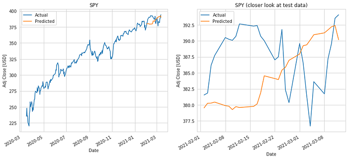
We test the model by inverse transforming the predictions made on the test dataset and comparing it to inverse transformed y_test values.

We ended up with a mean absolute error of $6.76 and a RMS error of $7.79. This seems to be slightly better than the linear regression predictions. In the next section, we will compare the two algorithms for different prediction windows.

Hyperparameter Tuning

We try to improve upon the base LSTM model by evaluating a range of values in the hyperparameter space using cross validation. For this, we use Keras Tuner.

We look at the following parameters: number of neurons in our first and second LSTM layers, dropout rate, number of dense layers as well as the number of neurons in each of them. For each of these we specify a range by providing the minimum value, the maximum value and the step size.

def build_model(hp):

    model = Sequential()

    model.add(LSTM(hp.Int('input_units',
                          min_value=32,
                          max_value=256,
                          step=32),
                   input_shape=(X_train.shape[1], X_train.shape[2]),
                   return_sequences=True))

    model.add(LSTM(hp.Int('secondary_units',
                          min_value=32,
                          max_value=128,
                          step=32),
                   return_sequences=False))

    model.add(Dropout(hp.Float('dropout', 0, 0.5, step=0.1)))

    for i in range(hp.Int('n_layers', 1, 2)):
        model.add(Dense(hp.Int(f'dense_{i}_units',
                               min_value=8,
                               max_value=32,
                               step=8)))

    model.add(Dense(y_train.shape[1]))

    model.compile(optimizer='adam', loss='mse', metrics=['mse'])

    return model

A random search is then performed to find the best hyperparameters that optimise the mean squared errror. We can find the best set of hyperparameters as follows:

tuner.get_best_hyperparameters()[0].values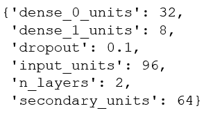

We use these hyperparameters to evaluate results of our LSTM model in the next section.

Results

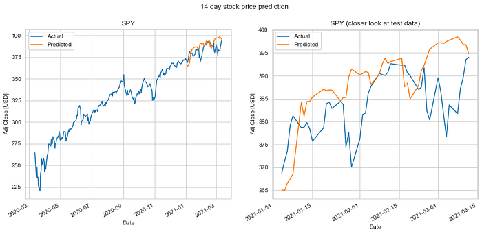
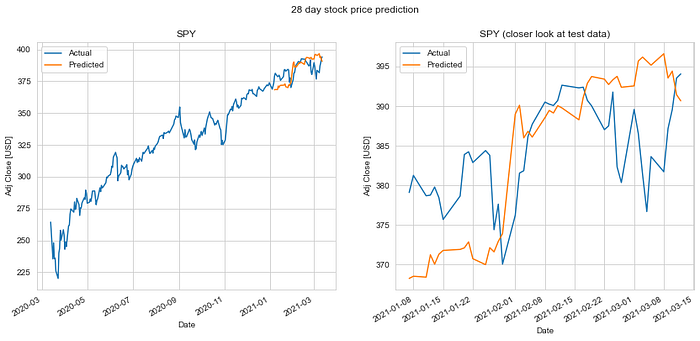
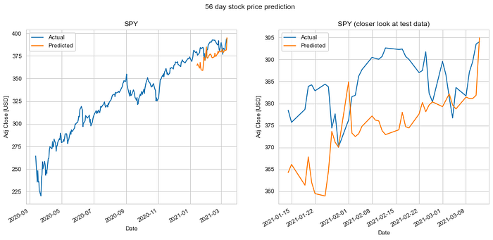
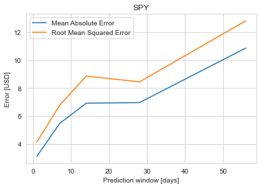
We do an 80%-20% train-test split on the data and evaluate it to predict stock price 1 day, 7 days, 14 days, 28 days and 56 days into the future. Keys metrics used are mean absolute error and RMS error.

The results of our test are summarized in the table. The mean absolute error in prediction for LSTM was 6.20% less than the mean absolute error of the predicitons made using Linear Regression (LR). And the RMS error for LSTM was 6.77% less than that of the LR predictions. Hence, LSTM would definitely be a better choice to predict stock price future value based on historical data. The plots for each of these runs are shown below for you to take a closer look at.

Note: For LSTM we used the best parameters obtained by hyperparameter tuning. Just as a recap in sequential order, we had 2 LSTM layers, a dropout layer and 3 dense layers. The first LSTM layer had 96 neurons and second had 64. The dropout layer had a dropout rate of 0.1. Finally, the first and second dense layers had 32 and 8 neurons respectively. The last dense layer was the output layer.

Linear Regression

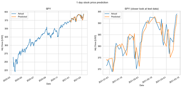
LSTM Neural Network

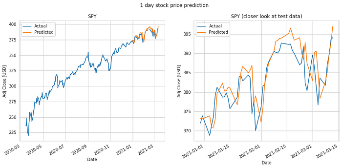
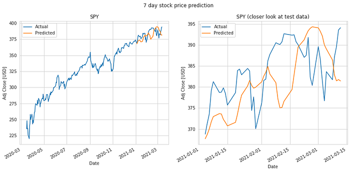
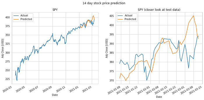
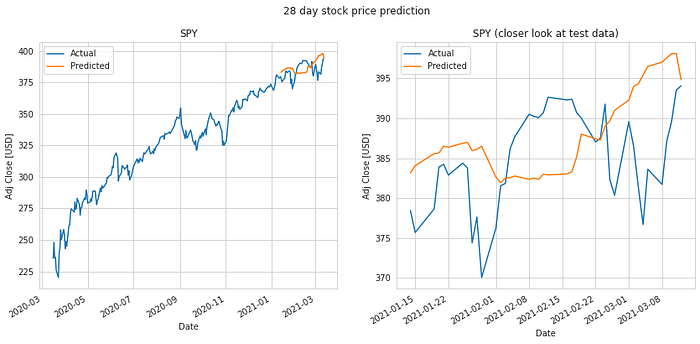
It is quite obvious from the above plotted results that the error in prediction increases as we increase our prediction time window. Moreover, LSTM does a better job at predicting longer term future stock price compared to the Linear Regression model. This can be attributed to the fact that the LSTM model looks at a series of historical data rather than a single point as in the case of Linear Regression model. Not just that, the ability of the neural network to backpropagate error and update weights results in a finely tuned model which better fits the data.

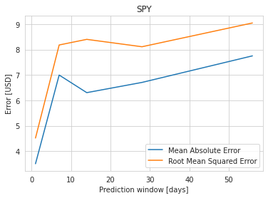
Linear regression error (left) vs LSTM error (right)

Looking at all these results, we may wondering if the model is useful in practical application with its current performance. We all would be rich if we could predict the market. The time series forecasting technique may work well with the momentum of the market. However, there’s always a possibility of a stock market crash due to a number of external factors which we cannot predict. This could be the starting point to build a more robust stock price predicter by doing some feature engineering and taking into account other factors such as news and quarterly company reports.

Conclusion

To summarize the work done, we obtained ‘SPY’ stock price data for last year and looked at regression as well as LSTM neural network to predict the stock price. For regression, linear regression did a good job, however decision tree regressor did not work well for time series forecasting. We then looked at LSTM neural network and compared its performance against linear regression after hyperparameter tuning. We were able to predict the ‘SPY’ stock price within ~2% error using the LSTM neural network.

As a trader and data scientist, I found this project pretty exciting to work on. However, I strongly discourage you all from using these techniques to trade in the stock market as there are a lot of factors which influence stock prices. Moreover, just cause our algorithm worked well for the ‘SPY’ stock, doesn’t mean it works well for other stocks. Here are a few suggestions to improve the prediction model:

Incorporating news sentiment. News has a big role in influencing stock price. Building a NLP model to classify news as good or bad will definitely help improve predictions.
It will be worth adding other technical factors such as moving average, momentum and bollinger bands to our set of features.
Finally, we should not ignore the fundamental factors of companies such as intrinsic value, book value and market capitalization. These are key to estimating the value of a company.

The code for this work can be found here.

“Rule #1: Don’t lose money.
Rule #2: Don’t forget Rule #1.” (Warren Buffett)